对数值类型的特征进行处理的方法,从而得到进行数据建模期望的特征值。
import numpy as np
import sklearn.preprocessing as prpr
1 二值法
1.1 noraml
X = np.array([[1,-1,2],
            [2,0,0],
             [0,1,-1]
             ])
X[X<=1]=0
X[X>1]=1
X
array([[0, 0, 1],
       [1, 0, 0],
       [0, 0, 0]])
1.2 Binarizer
Binarizer需要指定一个阈值threshold,当大于这个阈值时为1,否则为0
X = np.array([[1.0,-1,2],
            [2,0,0],
             [0,1.0,-1]
             ])
binarizer = prpr.Binarizer(threshold=1.0)
Xa = binarizer.transform(X)
Xa
array([[ 0.,  0.,  1.],
       [ 1.,  0.,  0.],
       [ 0.,  0.,  0.]])
2 取整(rounding)
X = np.array([[1.2,-1,2],
            [2,0,0],
             [0.9,1.9,-1]
             ])
Xb = np.round(X[:,0])
Xb
array([ 1., 2., 1.])
# 可以发现虽然去掉了小数点,但数组的元素类型依然为浮点型
np.array(Xb,dtype='int')
array([1, 2, 1])
3 iteraction
X = np.arange(6).reshape(3,2)
X
array([[0, 1],
       [2, 3],
       [4, 5]])
polyfeatures  = prpr.PolynomialFeatures(degree=2)
Xa = polyfeatures.fit_transform(X)
Xa
array([[  1.,   0.,   1.,   0.,   0.,   1.],
       [  1.,   2.,   3.,   4.,   6.,   9.],
       [  1.,   4.,   5.,  16.,  20.,  25.]])
PolynomialFeatures(degree=2,interaction_only=False, include_bias=False),生成的结果为 1, a,b,a^2,ab,b^2
4 Binning(quantization)量化
使用场景:
- 原始数据发生倾斜:即有些数据发生频率很高,有些却极少发生
- 倾斜的数据很容易造成建模时发生问题,例如,梯度下降有时会很慢
方法:
- fixed-width binning
- adaptive binning
4.1 fixed-width binning
import pandas as pd
fcc = pd.read_csv('datasets/2016-FCC-New-Coders-Survey-Data.csv',encoding='utf-8')
C:\Users\liuwu\Anaconda3\lib\site-packages\IPython\core\interactiveshell.py:2698: DtypeWarning: Columns (21,57) have mixed types. Specify dtype option on import or set low_memory=False.
  interactivity=interactivity, compiler=compiler, result=result)
fcc[['ID.x', 'EmploymentField', 'Age', 'Income']].head()
| ID.x | EmploymentField | Age | Income | |
|---|---|---|---|---|
| 0 | cef35615d61b202f1dc794ef2746df14 | office and administrative support | 28.0 | 32000.0 |
| 1 | 323e5a113644d18185c743c241407754 | food and beverage | 22.0 | 15000.0 |
| 2 | b29a1027e5cd062e654a63764157461d | finance | 19.0 | 48000.0 |
| 3 | 04a11e4bcb573a1261eb0d9948d32637 | arts, entertainment, sports, or media | 26.0 | 43000.0 |
| 4 | 9368291c93d5d5f5c8cdb1a575e18bec | education | 20.0 | 6000.0 |
visualize the data
import matplotlib.pyplot as plt
%matplotlib inline
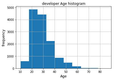
fig,ax = plt.subplots()
fcc['Age'].hist()
ax.set_title('developer Age histogram')
ax.set_xlabel('Age',fontsize=12)
ax.set_ylabel('frequency',fontsize=12)
Text(0,0.5,'frequency')
- 按照宽度均等的要求将数据放入不同的bin中
fcc['Age_bin_round'] = np.floor(fcc['Age']/ 10)
fcc[['ID.x', 'EmploymentField', 'Age', 'Income','Age_bin_round']].head()
| ID.x | EmploymentField | Age | Income | Age_bin_round | |
|---|---|---|---|---|---|
| 0 | cef35615d61b202f1dc794ef2746df14 | office and administrative support | 28.0 | 32000.0 | 2.0 |
| 1 | 323e5a113644d18185c743c241407754 | food and beverage | 22.0 | 15000.0 | 2.0 |
| 2 | b29a1027e5cd062e654a63764157461d | finance | 19.0 | 48000.0 | 1.0 |
| 3 | 04a11e4bcb573a1261eb0d9948d32637 | arts, entertainment, sports, or media | 26.0 | 43000.0 | 2.0 |
| 4 | 9368291c93d5d5f5c8cdb1a575e18bec | education | 20.0 | 6000.0 | 2.0 |
- 按照不同的宽度要求将数据放入到不同的bin中
bin_range=[0,15,30,45,60,70,100]
bin_label=[1,2,3,4,5,6]
fcc['Age_bin_range'] = pd.cut(fcc['Age'],bins=bin_range)
fcc['Age_bin_label'] = pd.cut(fcc['Age'],bins=bin_range,labels=bin_label)
fcc[['Age','Age_bin_round','Age_bin_range','Age_bin_label']].head(10)
| Age | Age_bin_round | Age_bin_range | Age_bin_label | |
|---|---|---|---|---|
| 0 | 28.0 | 2.0 | (15, 30] | 2 |
| 1 | 22.0 | 2.0 | (15, 30] | 2 |
| 2 | 19.0 | 1.0 | (15, 30] | 2 |
| 3 | 26.0 | 2.0 | (15, 30] | 2 |
| 4 | 20.0 | 2.0 | (15, 30] | 2 |
| 5 | 34.0 | 3.0 | (30, 45] | 3 |
| 6 | 23.0 | 2.0 | (15, 30] | 2 |
| 7 | 35.0 | 3.0 | (30, 45] | 3 |
| 8 | 33.0 | 3.0 | (30, 45] | 3 |
| 9 | 33.0 | 3.0 | (30, 45] | 3 |
fcc[['Age','Age_bin_round','Age_bin_range','Age_bin_label']].iloc[1071:1076]
| Age | Age_bin_round | Age_bin_range | Age_bin_label | |
|---|---|---|---|---|
| 1071 | 22.0 | 2.0 | (15, 30] | 2 |
| 1072 | 21.0 | 2.0 | (15, 30] | 2 |
| 1073 | 40.0 | 4.0 | (30, 45] | 3 |
| 1074 | 34.0 | 3.0 | (30, 45] | 3 |
| 1075 | 29.0 | 2.0 | (15, 30] | 2 |
4.2 adaptive binning
fix-width binning会导致有些bin会装很多数据,而有些bin只有少数数据甚至为空,依然无法解决数据偏斜的问题, adaptive binning是一种比fix-width更好更安全的方法,可以根据数据本身的分布将数据分到不同的bin中。
方法:
- 二分位
- 四分位
- 十分位
可视化数据
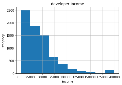
fig,ax = plt.subplots()
fcc['Income'].hist()
ax.set_title('developer income')
ax.set_xlabel('income')
ax.set_ylabel('freqency')
Text(0,0.5,'freqency')
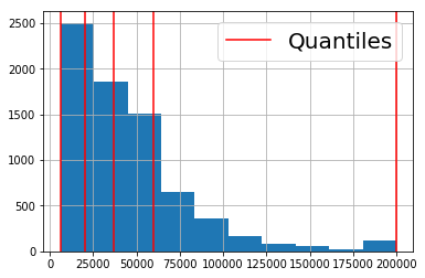
quantile_list=[0,0.25,0.5,0.75,1.0]
quat= fcc['Income'].quantile(quantile_list)
quat
0.00      6000.0
0.25     20000.0
0.50     37000.0
0.75     60000.0
1.00    200000.0
Name: Income, dtype: float64
# 可视化数据
fig,ax = plt.subplots()
fcc['Income'].hist()
for q in quat:
    plv = plt.axvline(q,color='r')
    ax.legend([plv],['Quantiles'],fontsize=20)
q_labels = ['0-25Q','25-50Q','50-75Q','75-100Q']
fcc['Income_q_range'] = pd.qcut(fcc['Income'],q=quantile_list)
fcc['Income_q_label'] = pd.qcut(fcc['Income'],q=quantile_list,labels=q_labels)
fcc[['Income','Income_q_range','Income_q_label']].head()
| Income | Income_q_range | Income_q_label | |
|---|---|---|---|
| 0 | 32000.0 | (20000.0, 37000.0] | 25-50Q |
| 1 | 15000.0 | (5999.999, 20000.0] | 0-25Q |
| 2 | 48000.0 | (37000.0, 60000.0] | 50-75Q |
| 3 | 43000.0 | (37000.0, 60000.0] | 50-75Q |
| 4 | 6000.0 | (5999.999, 20000.0] | 0-25Q |
5 Statistical Transformations
用于将数值型的特征的分布转化为尽量贴近正态分布(normal distribution)的特征。
5.1 Log Transform
fcc['Income_log'] = np.log(1 + fcc['Income'])
fcc_mean = np.round(np.mean(fcc['Income_log']),2)
fig, ax = plt.subplots()
fcc['Income_log'].hist()
plt.axvline(fcc_mean,color='red')
ax.set_xlabel('Income_log scale')
ax.set_ylabel('frequecy')
Text(0,0.5,'frequecy')
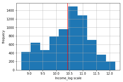
As we can see from the above figure, it is nearly close to the normal distribution but we can do much better.
let ‘s see how to do this with box-cox
5.2 box-cox transform
限制条件:
-
输入数字必须为正数;如果含有负数,使用常量lamda: $\lambda$ 将其转为正数如下:
-
如果$\lambda = 0 $,则为log transform
income = np.array(fcc['Income'])
income.shape
(15620,)
income_clean = income[~np.isnan(income)]
import scipy.stats as spstats
# 获取最优的lambda
l,opt_lambda = spstats.boxcox(income_clean)
print('optical lambda value is:',opt_lambda)
optical lambda value is: 0.117991226621
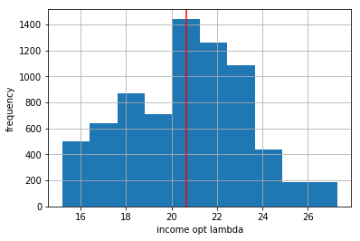
fcc['Income_lambda_0'] = spstats.boxcox((1+fcc['Income']),lmbda=0)
fcc['Income_lambda_opt'] = spstats.boxcox(fcc['Income'],lmbda=opt_lambda)
C:\Users\liuwu\Anaconda3\lib\site-packages\scipy\stats\morestats.py:1030: RuntimeWarning: invalid value encountered in less_equal
  if any(x <= 0):
visualization the data
fig,ax = plt.subplots()
plt.axvline(np.round(np.mean(fcc['Income_lambda_opt']),2),color='red')
fcc['Income_lambda_opt'].hist()
ax.set_xlabel('income opt lambda')
ax.set_ylabel('frequency')
Text(0,0.5,'frequency')