SVM is mainly forcus on the classification for the samples which are very close to the classifier boundary, while LR focus on the global samples to make them far away from the classifier boundary. There are 2 kinds of SVM:
- SVM without kernel(linear svm)
- when the \(\Theta * X >= 0\), y = 1; otherwise, y = 0
- classify the training set with linear line.
- SVM with kernel(typically gaussian kernel)
- used to classify the training set with nonlinear line
- the key is to choose the best C(\(\frac{1}{\lambda}\)) and sigma(\(\delta\))
load the data and visualization
    %matplotlib inline

    import numpy as np
    import scipy.io # used to import mat data
    import matplotlib.pyplot as plt # used to plot the data to visualize
    from sklearn import svm # the svn lib
load the data
    # load the data
    filename = 'ex6/data/ex6data1.mat'
    mat = scipy.io.loadmat(filename)
    X = mat['X']
    y = mat['y']
visualization
    # visualization
    def plotData(myX, myY):
        """
        plot the data:myX with label in myY
        """
        plt.figure(figsize=(8,6)) # create a new figure
        myY = myY.flatten()
        pos = myY==1
        neg = myY==0
        posX = myX[pos]
        negX = myX[neg]
        plt.plot(posX[:,0],posX[:,1],'k+')
        plt.plot(negX[:,0],negX[:,1],'yo')

    plotData(X,y)
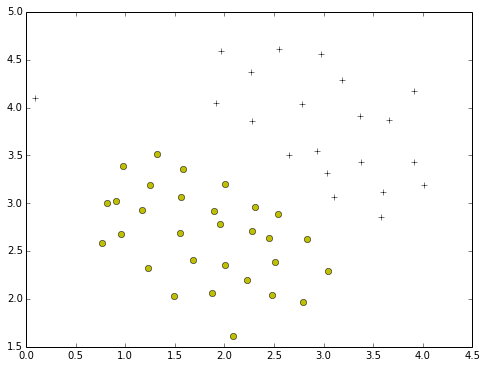
SVM without kernel to classify the data
SVM without kernel means it is a SVM with Linear
use SVM.svc to train
- with C=1.0
    train = svm.SVC(C=1.0,kernel='linear')
    train.fit(X,y.flatten())
    print train
Here is the description of the model:
    SVC(C=1.0, cache_size=200, class_weight=None, coef0=0.0,
      decision_function_shape=None, degree=3, gamma='auto', kernel='linear',
      max_iter=-1, probability=False, random_state=None, shrinking=True,
      tol=0.001, verbose=False)
plot the boundary
def plotBoundary(train,X):
b = train.intercept_[0] # the bias
theta = train.coef_[0] # the weight
#print type(theta),theta.shape
x1 = np.insert(X[:,:-1],0,1,axis=1)
theta = np.insert(theta,0,b)
#print theta
x2 = np.dot(x1, theta[:-1].T) / -theta[-1]
#print x2[:10],x2.shape,x1.shape
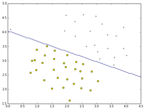
plt.plot(x1[:,1],x2,'b-')
plotData(X,y)
plotBoundary(train,X)
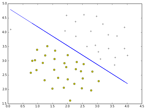
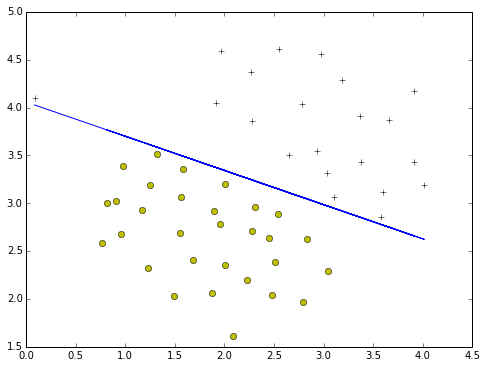
- C=10.0
    train = svm.SVC(C=100,kernel='linear')
    train.fit(X,y.flatten())

    plotData(X,y)
    plotBoundary(train,X)
    def plotBoundary2(mySVM, xmin, xmax, ymin, ymax):
        """
        Function to plot the decision boundary for a trained SVM with 2-n sample data
        """
        xvals = np.linspace(xmin, xmax,100)
        yvals = np.linspace(ymin, ymax,100)
        zvals = np.zeros((len(xvals),len(yvals)))
        for i in xrange(len(xvals)):
            for j in xrange(len(yvals)):
                zvals[i][j] = float(mySVM.predict(np.array([[xvals[i],yvals[j]]]))[0])
        zvals = zvals.transpose()
        u, v = np.meshgrid( xvals, yvals )
        plt.contour(xvals,yvals,zvals,[0])
    plotData(X,y)
    plotBoundary2(train,0,4.5,1.5,5)
Gaussian Kernels
SVM without kernel is a linear classifier, but when we want to have a nonlinear classifier, we need to make use of kernel to help
the formula
    def gaussianKernel(x1,x2, delta):
        """
        function used to compute the gaussian possibility
        """
        t = x1 - x2
        return np.exp(-np.dot(t.T,t) / (2.0 * np.power(delta,2)))

    x1 = np.array([1, 2, 1])
    x2 = np.array([0, 4, -1])
    sigma = 2

    print "the expected result should be:0.324652, and the real output is:%0.6f" % gaussianKernel(x1,x2,sigma)
here we come to the following result:
the expected result should be:0.324652, and the real output is:0.324652
load the data and visualization
    filename = 'ex6/data/ex6data2.mat'
    mat = scipy.io.loadmat(filename)
    X = mat['X']
    y = mat['y']

    plotData(X,y)
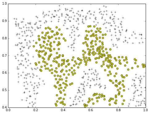
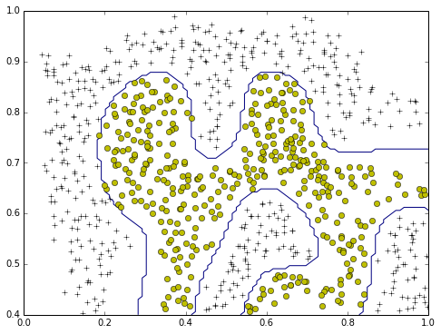
use rbf to train the model
    C,sigma = 1,0.1
    train = svm.SVC(C=C,kernel='rbf',gamma=100.0)
    train.fit(X,y.flatten())
    print train
here is the description of the model:
    SVC(C=1, cache_size=200, class_weight=None, coef0=0.0,
      decision_function_shape=None, degree=3, gamma=100.0, kernel='rbf',
      max_iter=-1, probability=False, random_state=None, shrinking=True,
      tol=0.001, verbose=False)
    plotData(X,y)
    plotBoundary2(train,0,1.0,0.4,1.0)
Cross-validation to choose the best C and sigma
load the data3
    filename = 'ex6/data/ex6data3.mat'
    mat = scipy.io.loadmat(filename)
    X = mat['X']
    y = mat['y']
    Xval = mat['Xval']
    yval = mat['yval']
choose C and sigma
    def evaluateSVM(X,y,Xval,yval):
        """
        function used to compute the best C and sigma for the SVC model using parameter:<X,y> as training set,
        and <Xval, yval> as the validation set
        """
        T = [0.01,0.03,0.1,0.3,1,3,10,30] # this is used for the candidate number for both C and sigma
        score= 0.0
        C,gamma=0.0,0.0

        for c in T:
            for delta in T:
                sigma = np.power(delta,-2.0)
                model = svm.SVC(C=c,kernel='rbf',gamma=sigma)
                model.fit(X,y.flatten())

                # predict
                ypred = model.predict(Xval)
                sc = float(np.sum(yval.flatten()==ypred)) / len(yval)
                if (sc > score):
                    score = sc
                    #print score
                    C = c
                    gamma = sigma

        return C,gamma

    C,gamma = evaluateSVM(X,y,Xval,yval)
    print "Best C=%f, Best gamma=%f" % (C,gamma)
Now, we come to result:
Best C=0.300000, Best gamma=100.000000
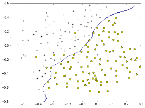
    model = svm.SVC(C=C,kernel='rbf',gamma=gamma)
    model.fit(X,y.flatten())
    plotData(X,y)
    plotBoundary2(model,-0.5,0.3,-0.8,0.6)