This blog we’re going to talk about principal compononent analysis to compress the original data, PCA is used to reduce the dimension of the samples.
feature normalization
import modules
    # import needed modules
    %matplotlib inline
    import numpy as np
    import matplotlib.pyplot as plt
    import scipy.io #Used to load the OCTAVE *.mat files
    import scipy.misc #Used to show matrix as an image
    import scipy.linalg
    from scipy import optimize
    import random
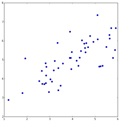
load the data
    fileName = 'ex7/data/ex7data1.mat'
    mat = scipy.io.loadmat(fileName)
    X = mat['X']

    plt.figure(figsize=(8,8))
    plt.plot(X[:,0],X[:,1],'bo')
    plt.show()
feature normalization
def featureNormalize(myX):
"""
normalize the features, return mean, standard deviration and normalized features
"""
mu = np.mean(myX, axis = 0)
dev = np.std(myX, axis = 0)
normX = (myX - mu)/dev
return (mu,dev,normX)
def getUSV(myX_norm):
"""
Singular value decomposition. Factorize a matrix into 2 unitary U and V
and a 1-D array s of singular values (real, non-negative) such that a == U*S*Vh,
where S is a suitably shaped matrix of zeros with main diagonal s.
"""
cov = np.dot(myX_norm.T,myX_norm) / myX_norm.shape[0]
return scipy.linalg.svd(cov)
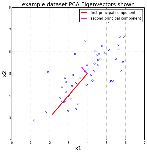
(mu,dev,normX) = featureNormalize(X)
(U,s,V) = getUSV(normX)
#print "top principal component is:", U[:,0]
plt.figure(figsize=(8,8))
plot = plt.scatter(X[:,0],X[:,1],s=30,facecolors='none',edgecolors='b')
plt.title("example dataset:PCA Eigenvectors shown", fontsize=18)
plt.xlabel('x1',fontsize=18)
plt.ylabel('x2',fontsize=18)
plt.grid(True)
plt.plot([mu[0], mu[0] + 1.5*s[0]*U[0,0]],
[mu[1], mu[1] + 1.5*s[0]*U[0,1]],
color='red',linewidth=3,label='first principal component')
plt.plot([mu[0], mu[0] + 1.5*s[1]*U[1,0]],
[mu[1], mu[1] + 1.5*s[1]*U[1,1]],
color='fuchsia',linewidth=3,label='second principal component')
plt.legend()
plt.show()
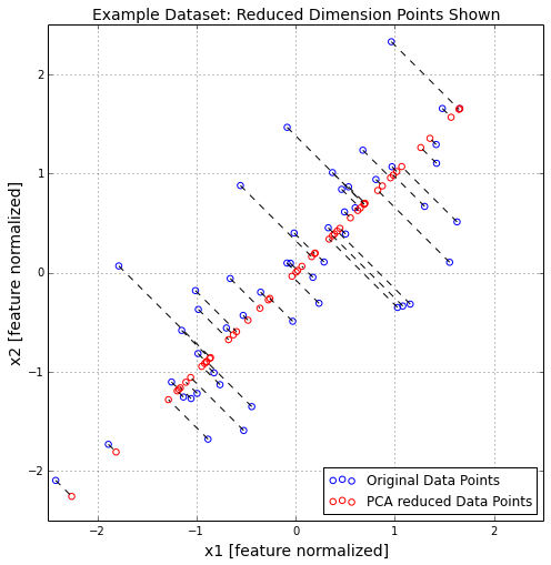
project the normalize data
    def projectData(X_norm, U, K):
        """
        computes the reduced data representation when projecting only
        X_norm: the normalized data
        U:
        K:the first K columns of U
        """
        return np.dot(X_norm,U[:,:K])

    Z = projectData(normX,U,1)
    print "Project of the first example:%f" % Z[0]


    Project of the first example:1.496313


    def recoverData(myZ, myU, K):
        return np.dot(myZ, myU[:,:K].T)

    X_rec = recoverData(Z,U,1)
    print "Recovered approximation of the first example is ",X_rec[0]
Recovered approximation of the first example is [-1.05805279 -1.05805279]
display
    plt.figure(figsize=(8,8))
    plt.scatter(normX[:,0],normX[:,1],s=30,facecolors='none',
                edgecolors='b',label='Original Data Points')
    plt.scatter(X_rec[:,0],X_rec[:,1],s=30,facecolors='none',
                edgecolors='r',label='PCA reduced Data Points')
    plt.title("Example Dataset: Reduced Dimension Points Shown",fontsize=14)
    plt.xlabel('x1 [feature normalized]',fontsize=14)
    plt.ylabel('x2 [feature normalized]',fontsize=14)
    plt.grid(True)
    for x in xrange(normX.shape[0]):
        plt.plot([normX[x,0],X_rec[x,0]],[normX[x,1],X_rec[x,1]],'k--')
    leg = plt.legend(loc=4)
    dummy = plt.xlim((-2.5,2.5))
    dummy = plt.ylim((-2.5,2.5))

    plt.show()
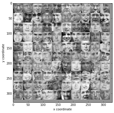
Use PCA to compress images
display the data
    import Utils4KMeans as CKM # import the needed modules for Kmeans
    import matplotlib.cm as cm #Used to display images in a specific colormap

    fileName = 'ex7/data/ex7faces.mat'
    mat = scipy.io.loadmat(fileName)
    X = mat['X']

    print X.shape
(5000, 1024)
    def getDatumImg(row):
        """
        Function that is handed a single np array with
        shape 1 * 1024, create an image object from it and return
        """
        width = int(np.sqrt(len(row)))
        height = width

        return row.reshape(width, height)

    def displayData(myX, mynrows=10, myncols =10):
        """
        Function that picks the first 100 rows from
        """
        width = int(np.sqrt(len(myX[0])))
        xPixes, yPixes = (width, width)
        nrows,ncols = (mynrows,myncols)
        pad = 1

        # this variable is used to store all the 100 samples data which are used to visualize
        big_pic = np.zeros((nrows * (xPixes + pad),ncols * (yPixes + pad)))

        cr,cl=(0,0) #cr stands for rows, cl stands for column
        for i in xrange(nrows):
            for j in xrange(ncols):
                # extract an sample as a 20 * 20 matrix
                sample = myX[i*nrows + j]#random.sample(myX,1) #randomly get a sample
                sample = np.array(sample).reshape(xPixes,yPixes) # ignore the first column with value 1

                big_pic[i * xPixes+pad:(i+1)*xPixes+pad,j*yPixes+pad:(j+1)*yPixes+pad] = sample.T

        plt.figure(figsize=(6,6))
        img = scipy.misc.toimage(big_pic)
        plt.xlabel('x coordinate')
        plt.ylabel('y coordinate')
        plt.imshow(img,cmap=cm.Greys_r)

    displayData(X[:100])
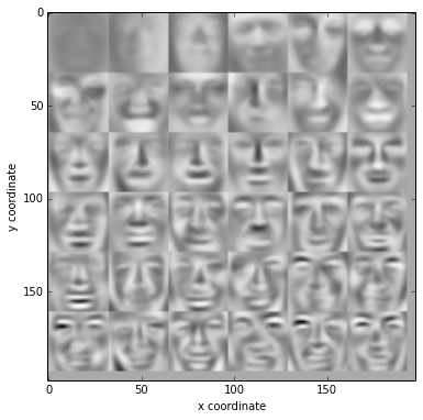
    (mean, std,normX) = featureNormalize(X)
    (U,s,V) = getUSV(normX)

    displayData(U[:,:36].T,6,6)
display the compressed images
    Z = projectData(normX,U,200)
    print "The projected data Z has a size of:",Z.shape[0]

    The projected data Z has a size of: 5000

    recX = recoverData(Z, U, 200)
    displayData(recX[:100])

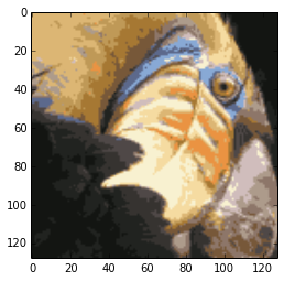
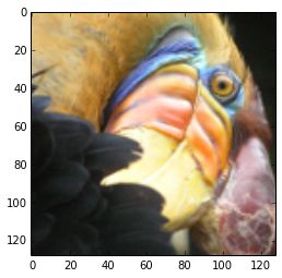
Use KMeans to compress the bird image
load the bird and display
    filename = 'ex7/data/bird_small.png'

    imgbird = scipy.misc.imread(filename)

    print "the bird image's shape:",imgbird.shape

    plt.figure()
    plt.imshow(imgbird)
    plt.show()
the bird image’s shape: (128, 128, 3)
normalize and compress
    X = imgbird.reshape(-1,3)
    X = X/255.0  # normalize the sample into range[0,1]

    myK = 16   # 16 centroid points
    init_cent = random.sample(X,myK)

    (ids,cent_history) = CKM.calMeanK(X,init_cent,maxIter=50)

    final_ids = CKM.findClosedCentroid(X,cent_history[-1])

    final_cent = cent_history[-1]
    compressed_X = np.array([final_cent[i] for i in final_ids.flatten()])
    compressed_X = compressed_X.reshape(imgbird.shape)

    plt.figure()
    plt.imshow(compressed_X)
    plt.show()