Overview
Implement Logistic Regression Using IPython notebook
Logistic Regression without regularization
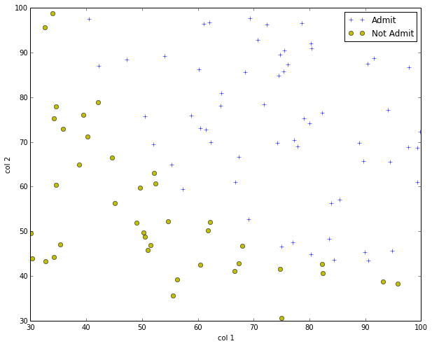
visualize the data
import modules numpy and matplotlib
# build in the pyplot into notebook
%matplotlib inline
import numpy as np
import matplotlib.pyplot as plt
import the sample data from the files
fileName = 'ex2/data/ex2data1.txt'
cols = np.loadtxt(fileName, np.float, delimiter=',',usecols=(0,1,2),unpack=True)
X = cols[:-1].T
Y = cols[-1:].T
X = np.insert(X, 0, 1, axis=1) #axis = 1 means to insert the 1 before column index:0; it axis = 0, insert before the row index:0

posX = np.array([X[i] for i in xrange(len(X)) if Y[i][0]==1])
negX = np.array([X[i] for i in xrange(len(X)) if Y[i][0]==0])
visulization the samples
def plotData(X, Y):

    # filter to get positive and negative examples
    plt.figure(figsize=(10,8))    # create a figure canvas
    plt.plot(posX[:,1],posX[:,-1],'+',label='Admit')
    plt.plot(negX[:,1],negX[:,-1],'yo',label='Not Admit')
    plt.xlabel('col 1')
    plt.ylabel('col 2')
    plt.legend()


plotData(X,Y)
plt.show()
Use sigmoid function to separate the data
the activation function
\(g(x)=\frac{1}{1+e^{-z}}\)
其中 \(z = X \Theta\)
当\(z >= 0\)时, \(g(x) >= 0.5\)
当\(z < 0 \)时, \(g(x) < 0.5\)
the loss function
\(J(\theta) = \frac{1}{m} \sum_{i=1}^{m}[-y^i log(h_{\theta}(x^i)) - (1 - y^i) log(1 - h_{\theta}(x^i))]\)
the gradient of the cost:
\(\frac{\partial J(\theta))}{\partial \theta_j} = \frac{1}{m} \sum_{i=1}^{m}(h_{\theta}(x^i) - y^i)x_j^i\)
implementation using sigmoid function
    # define the iteration = 400
    iterations = 400
    # define the init_theta = 0
    init_theta = np.zeros((X.shape[1],1))

    # import the module optimize from SciPy
    from scipy import optimize

    def f(z):
        return 1.0/(1 + np.exp(-z))

    def costFunction(theta, X, Y, mylambda=0.0):
        theta = theta.reshape(-1,1)
        Z = np.dot(X,theta)
        T = f(Z)
        result = np.sum(Y * np.log(T) + (1 - Y)*np.log(1-T)) * (-1) / len(X)
        if np.isnan(result):
            return np.inf
        return result

    def gradient(theta, X, Y):
        theta = theta.reshape(-1,1)
        #print theta, theta.shape
        Z = np.dot(X, theta)   # m*1
        T = f(Z)
        result = np.dot(X.T,T - Y) / len(X)  # n * 1
        return result.flatten()

    costFunction(init_theta,X,Y)
0.69314718055994584
    theta = init_theta
    print theta.shape
    result = optimize.minimize(costFunction,theta,args=(X,Y),method='BFGS',jac=gradient, options={'maxiter':400})
    print result
(3, 1)
status: 0
success: True
njev: 30
nfev: 30
hess_inv: array([[ 3.07660923e+03, -2.46603141e+01, -2.46347979e+01],
[ -2.46603141e+01, 2.11901191e-01, 1.84691126e-01],
[ -2.46347979e+01, 1.84691126e-01, 2.12563326e-01]])
fun: 0.20349770158966385
x: array([-25.16136291, 0.20623191, 0.20147189])
message: ‘Optimization terminated successfully.’
jac: array([ 5.11757491e-08, 2.27330775e-06, 5.15598733e-06])
costFunction(result.x,X,Y)
0.20349770158966385
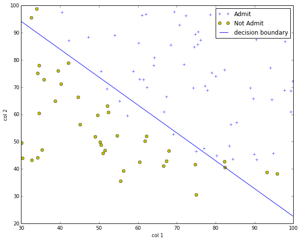
visualize the boundary
    plotData(X,Y)

    theta = result.x
    boundary_x = np.array([np.min(X[:,1]),np.max(X[:,1])]) # x boundary
    boundary_y = (boundary_x * theta[1] + theta[0]) * (-1.0)/theta[2]
    plt.plot(boundary_x, boundary_y, 'b-',label='decision boundary')

    plt.legend()
    plt.show()
predict precision
    def makePredict(theta, X):
        return f(np.dot(X, theta.reshape(-1,1))) >=0.5

    pos_count = float(np.sum(makePredict(theta, posX)))
    neg_count = float(np.sum(np.invert(makePredict(theta,negX))))

    print "Fraction of training samples correctly predicted: %f." % ((pos_count + neg_count) / (len(posX) + len(negX)))
Fraction of training samples correctly predicted: 0.890000.
logistic regression with regularization
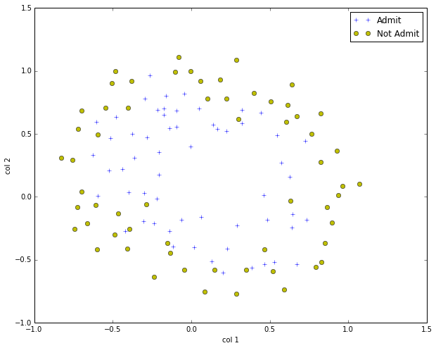
visualize the sample data
extract data from the txt file
    fileName = 'ex2/data/ex2data2.txt'
    cols = np.loadtxt(fileName, np.float, delimiter=',',usecols=(0,1,2),unpack=True)
    X = cols[:-1].T
    Y = cols[-1:].T
    X = np.insert(X, 0, 1, axis=1) #axis = 1 means to insert the 1 before column index:0; it axis = 0, insert before the row index:0

    posX = np.array([X[i] for i in xrange(len(X)) if Y[i][0]==1])
    negX = np.array([X[i] for i in xrange(len(X)) if Y[i][0]==0])

    plotData(X,Y)
map the features
    def mapFeatures(col1, col2):
        degree = 6
        m = len(col1)
        out = np.ones((m,1))
        for i in xrange(1, degree+1):
            for j in xrange(0, i+1):
                term1 = col1 ** (i-j)
                term2 = col2 ** j
                term = (term1 * term2)
                # print term.shape
                term = term.reshape((m,1))
                out = np.hstack((out,term))
        return out

    mappedX = mapFeatures(X[:,1],X[:,-1])
    print mappedX
The output is:
    [[  1.00000000e+00   5.12670000e-02   6.99560000e-01 ...,   6.29470940e-04
        8.58939846e-03   1.17205992e-01]
     [  1.00000000e+00  -9.27420000e-02   6.84940000e-01 ...,   1.89305413e-03
       -1.39810280e-02   1.03255971e-01]
     [  1.00000000e+00  -2.13710000e-01   6.92250000e-01 ...,   1.04882142e-02
       -3.39734512e-02   1.10046893e-01]
     ...,
     [  1.00000000e+00  -4.84450000e-01   9.99270000e-01 ...,   2.34007252e-01
       -4.82684337e-01   9.95627986e-01]
     [  1.00000000e+00  -6.33640000e-03   9.99270000e-01 ...,   4.00328554e-05
       -6.31330588e-03   9.95627986e-01]
     [  1.00000000e+00   6.32650000e-01  -3.06120000e-02 ...,   3.51474517e-07
       -1.70067777e-08   8.22905998e-10]]
formula with regularization
\(J(\theta) = \frac{1}{m} \sum_{i=1}^{m}[-y^i log(h_{\theta}(x^i)) - (1 - y^i) log(1 - h_{\theta}(x^i))] + \frac{\lambda}{2m} \sum_{j=1}^{m}\theta_j^2\)
the gradient of the cost:
\(\frac{\partial J(\theta))}{\partial \theta_0} = \frac{1}{m} \sum_{i=1}^{m}(h_{\theta}(x^i) - y^i)x_0^i\) for \(j=0\)
\(\frac{\partial J(\theta))}{\partial \theta_j} = \frac{1}{m} \sum_{i=1}^{m}(h_{\theta}(x^i) - y^i)x_j^i + \frac{\lambda}{m} \theta_j\) for \(j=1,2,\cdots,n\)
implementation
    def costFunctionWithReg(theta, X, Y, mylambda=0.0):
        theta = theta.reshape(-1,1)
        Z = np.dot(X,theta)
        T = f(Z)
        m = len(X)
        result = np.sum(Y * np.log(T) + (1 - Y)*np.log(1-T)) * (-1) / len(X)
        theta2 = theta[1:,:]
        result = result + (mylambda / (2* m)) * np.dot(theta2.T,theta2)
        if np.isnan(result):
            return np.inf
        return result

    def gradientWithReg(theta, X, Y, mylambda = 0.0):
        theta = theta.reshape(-1,1)
       # print theta, theta.shape
        Z = np.dot(X, theta)   # m*1
        T = f(Z)
        m = len(X)
        result = np.dot(X.T,T - Y) / len(X)  # n * 1
        theta[0] = 0
        result = result + (mylambda / m) * theta
        return result.flatten()

    result = optimize.minimize(costFunctionWithReg, np.zeros((mappedX.shape[1],1)), args=(mappedX,Y,0.0), method='BFGS',
                               jac=gradientWithReg,options={'maxiter':500,'disp':True})
Now come to the result:
    Warning: Maximum number of iterations has been exceeded.
             Current function value: 0.238242
             Iterations: 500
             Function evaluations: 501
             Gradient evaluations: 501
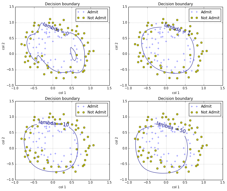
plot the boundary with different lambda
def plotMultiVariBoundary(myX, myY, mylambda=0.0):
    result =optimize.minimize(costFunctionWithReg, np.zeros((mappedX.shape[1],1)), args=(mappedX,Y,mylambda), method='BFGS',
                           jac=gradientWithReg,options={'maxiter':500,'disp':True})
    theta = result.x
    minCost = result.fun
    xvals = np.linspace(-1,1.5,50)
    yvals = np.linspace(-1,1.5,50)
    zvals = np.zeros((len(xvals),len(yvals)))
    for i in xrange((len(xvals))):
        for j in xrange(len(yvals)):
            myfeaturesij = mapFeatures(np.array([xvals[i]]),np.array([yvals[j]]))
            zvals[i][j]=np.dot(theta,myfeaturesij.T)
    zvals = zvals.transpose()

    u,v = np.meshgrid(xvals, yvals)
    mycontour = plt.contour(xvals, yvals, zvals,[0])
    myfmt = {0:'lambda = %d' % mylambda}
    plt.clabel(mycontour,inline=1,fontsize=15,fmt=myfmt)
    plt.title("Decision boundary")

def plotData2():
    #plt.figure(figsize=(10,8))    # create a figure canvas
    plt.plot(posX[:,1],posX[:,-1],'+',label='Admit')
    plt.plot(negX[:,1],negX[:,-1],'yo',label='Not Admit')
    plt.xlabel('col 1')
    plt.ylabel('col 2')
    plt.legend()
    plt.grid(True)

# start to plot the data and boundary
plt.figure(figsize=(12,10))
plt.subplot(221)
plotData2()
plotMultiVariBoundary(X,Y,0.0)

plt.subplot(222)
plotData2()
plotMultiVariBoundary(X,Y,1.0)

plt.subplot(223)
plotData2()
plotMultiVariBoundary(X,Y,10.0)

plt.subplot(224)
plotData2()
plotMultiVariBoundary(X,Y,50.0)


Warning: Maximum number of iterations has been exceeded.
         Current function value: 0.238242
         Iterations: 500
         Function evaluations: 501
         Gradient evaluations: 501
Optimization terminated successfully.
         Current function value: 0.529003
         Iterations: 47
         Function evaluations: 48
         Gradient evaluations: 48
Optimization terminated successfully.
         Current function value: 0.648216
         Iterations: 21
         Function evaluations: 22
         Gradient evaluations: 22
Optimization terminated successfully.
         Current function value: 0.680722
         Iterations: 10
         Function evaluations: 11
         Gradient evaluations: 11